What does it mean to change an elasticity?
How would changing housing supply elasticities affect output? If AI induces a change in capital’s share of income, will that affect short-run growth and steady-state income per capita? These types of questions have been approached by performing “change elasticity” counterfactuals in quantitative models. They sound straightforward (indeed, I perform one in my JMP): we shock TFP all the time, so why can’t we change other parts of the production technology? It turns out that these counterfactuals aren’t really well-defined absent additional structure or shocks. Elasticities govern how parts of an economic system react to changes. A better posed question might be, how much larger would economic growth have been had housing supply elasticities been higher? For a given quantified model, however, changing elasticities and holding all else fixed can induce changes that depend arbitrarily on the units of the data to which the model was calibrated.
Greaney (2026) clarifies these scale-dependence issues as they arise in the counterfactuals of Hsieh and Moretti (2019). Recently, Rachel (2026) makes the same point for counterfactuals in which capital’s share of income changed: a seemingly innocuous productivity normalization can determine the gains from “automation.”
I try to explain these issues in this post. Almost none of what follows is new. The point of this post is to hammer them home and outline what researchers can do, instead.
First, I walk through a single-market housing example with an isoelastic supply curve. Then I show these exact issues arise in a dynamic model – the neoclassical growth model – when changing capital’s share of income.
I’m also attaching a short PDF that walks through these models in detail for the interested researcher. While I would be happy with the citation, Greaney (2026) deserves it more.
A housing example
I now ask what the welfare effects are from changing a housing supply elasticity in a simple model of the housing market. Suppose households consume a numeraire good $C$ and housing $H$,
\[\max_{C,H} C^{1-\beta}H^\beta \quad\text{s.t.}\quad C+pH\leq M,\]where $0<\beta<1$ and $M$ is exogenous income. Housing supply is $H=Sp^\gamma$, with $S>0$ and $\gamma\geq0$. For now, households do not receive housing profits (in the PDF appendix I work this out). Market clearing is given by $pH=\beta M$, so equilibrium price and indirect utility are,
\[p=\left(\frac{\beta M}{S}\right)^{1/(1+\gamma)}, \qquad V=B\frac{M}{p^\beta}, \qquad B=(1-\beta)^{1-\beta}\beta^\beta.\]In practice, we don’t observe $S$, the “intercept” of the housing supply curve. Given $\beta$ and an assumed $\gamma_0$, we calibrate it from observed income and price:
\[S_0=\frac{\beta M_0}{p_0^{1+\gamma_0}}.\]Now change $\gamma$, holding income and the fitted $S$ fixed. How does welfare change? With $\hat V=V_1/V_0$,
\[\hat V=p_0^{\frac{\beta(\gamma_1-\gamma_0)}{1+\gamma_1}},\]as holding all else fixed, it must be that, $p_1^{1+\gamma_1} = p_0^{1+\gamma_0}$ so $\hat p = p_0^{-{\gamma_1 - \gamma_0 \over 1 + \gamma_1}}$. Raising the elasticity raises welfare if $p_0>1$ and lowers it if $p_0<1$. But whether a price exceeds one depends on the units!
Suppose $M_0$ is 100 dollars, $p_0$ is one dollar, $\beta=0.3$, and $\gamma_0=0.9$. Calibration gives $S_0=30$. Raising $\gamma$ to 1.8 does nothing: both supply curves pass through $p=1$, $H=30$, since $1^{0.9}=1^{1.8}=1$. Price and consumption stay fixed, so $\hat V=1$.
Now, let’s repeat the calculation at 100 yen per dollar. The same data are $M_0=10{,}000$ and $p_0=100$, and now $S_0=0.3\times10{,}000/100^{1.9}$. Raising $\gamma$ to 1.8 with this fitted coefficient fixed gives,
\[\hat V=100^{0.3(1.8-0.9)/2.8}=1.5590.\]Value utility at baseline prices. The welfare gain is worth $M_0(\hat V-1)$, or 5,590 yen. Converting back gives 55.90 dollars, versus zero when we do the calculation in dollars. Expressing the data in yen instead of dollars gives a different answer.
The problem is that holding each fitted $S$ fixed at $S_0$ chooses different counterfactual supply curves. The units of $S_0=\frac{\beta M_0}{p_0^{1+\gamma_0}}$ depend on $\gamma_0$; the units of $M_0$ and $p_0$ only cancel when $\gamma=0$! Freezing the value of $S$ is not an innocuous assumption about technology. If $S$ is recalibrated under $\gamma_1$, then nothing should change.
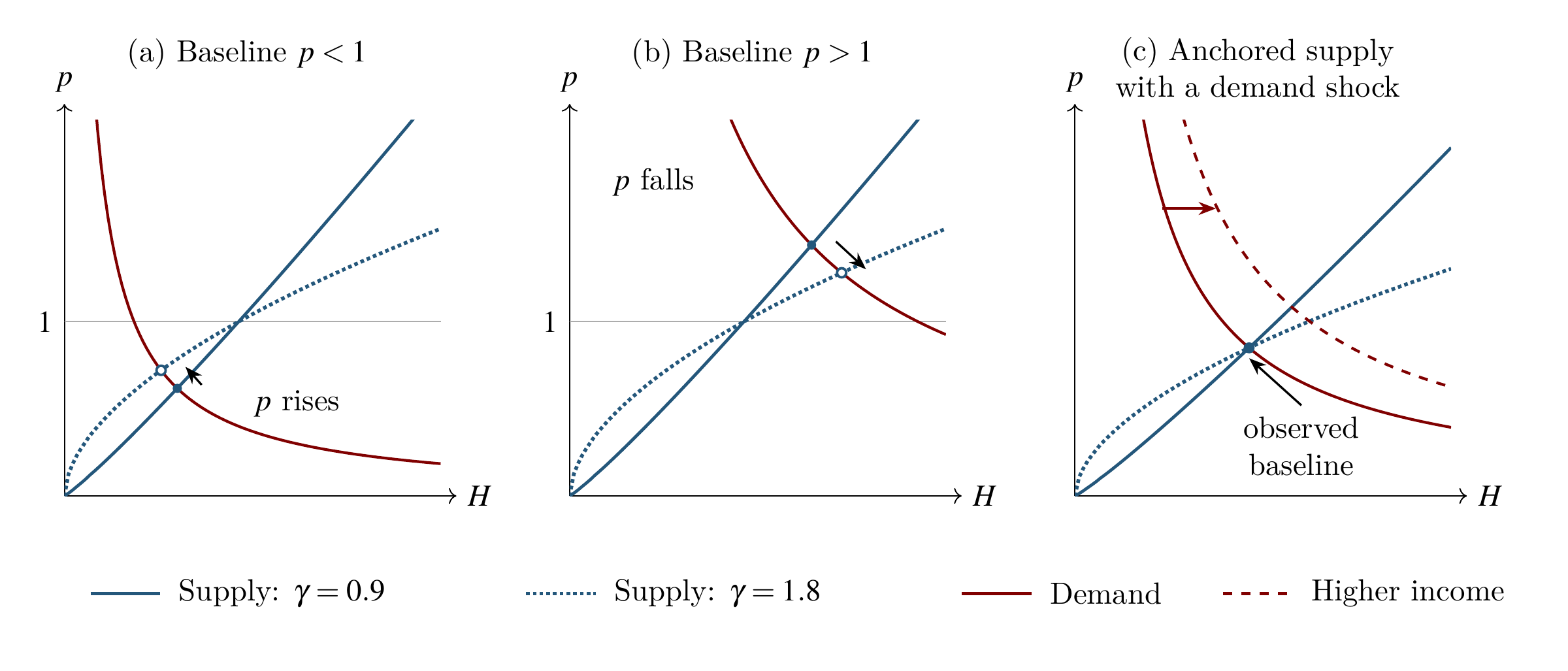
In (a) and (b), $S$ stays fixed as the elasticity rises. Whether price rises or falls depends on whether baseline price is below or above one.
In (c), both supply curves pass through the observed equilibrium, so changing $\gamma$ does nothing.
What to do instead
Following the price theory logic of panel (c), changing $\gamma$ changes nothing except for how the system reacts to a demand shock, pictured by the demand curve shifting out. Anchoring to the observed equilibrium – here, recalibrating $S$ to $\gamma_1$ – means that “change elasticity” counterfactuals, in this context, only make sense when paired with another shock.
To kick a dead horse: since elasticities change how a system reacts to shocks, it’s natural to compare how a system would react to the same shock with different technology. The recipe for this comparison is to “anchor” to an observed equilibrium (as in panel (c)), then feed in a shock under different elasticities.
In the housing example, for each $\gamma$, first fit the model to the observed equilibrium. Then raise income by 10%, keeping that model’s $S$ and $\gamma$ fixed:
\[S_0(\gamma)=\frac{\beta M_0}{p_0^{1+\gamma}}, \qquad \hat p=1.1^{1/(1+\gamma)}, \qquad \hat V=1.1^{1-\beta/(1+\gamma)}.\]With $\beta=0.3$, welfare rises by 8.36% at $\gamma=0.9$ and 8.88% at $\gamma=1.8$. As expected: more elastic supply dampens the price increase brought about by the income shock. Now, these answers don’t depend on dollars versus yen.
The key is refitting $S$. This is what makes all supply curves pass through the observed equilibrium – this is “anchoring.”
Changing capital’s share
The same issue appears in changing capital’s share of income, $\alpha$ in the neoclassical growth model. Suppose production technology is Cobb-Douglas, $y=Ak^\alpha$, where $y$ is income per worker and $k$ is capital per worker and we keep labor supply fixed. In what follows, I also assume log utility, discount factor 0.95, full capital depreciation, and a unit population inelastically supplying labor for tractability. Optimal saving is then $k_{t+1}=0.95\alpha y_t$.
Fitting the baseline. Suppose we observe only output per worker $y_0$. To infer capital, assume the baseline is in steady state. Given $\alpha_0$, calibration gives,
\[k_0=0.95\alpha_0 y_0, \qquad A_0=\frac{y_0}{k_0^{\alpha_0}}.\]We infer $k_0$ once, at the baseline $\alpha_0$. If we observe capital $k_0$ directly, we can instead fit $A_0$ off steady-state, but the units issues below will remain.
Now, let’s express income in yen at $\mathcal E$ yen per dollar. Here, with output as the numeraire, capital is measured in dollars and also multiplies by $\mathcal E$, and the fitted TFP value becomes $A_0^{\mathrm{yen}}=\mathcal E^{1-\alpha_0}A_0^{$}$. Both calibrations describe the same baseline economy.
Changing the technology. Now unexpectedly raise $\alpha$ to $\alpha_1$, keeping each fitted $A$ fixed at $A_0^{$}$ or $A_0^\text{yen}$. Let $y_{\mathrm{CF}}$ denote output immediately after the change and $\Delta\alpha=\alpha_1-\alpha_0$.
On impact, the predicted output changes are,
\[\frac{y_{\mathrm{CF}}^{\$}}{y_0^{\$}}-1 =(k_0^{\$})^{\Delta\alpha}-1, \qquad \frac{y_{\mathrm{CF}}^{\mathrm{yen}}}{y_0^{\mathrm{yen}}}-1 =(\mathcal E k_0^{\$})^{\Delta\alpha}-1.\]For example, with baseline income of 50 cents and $\alpha_0=0.3$, inferred capital is 14.25 cents, or 14.25 yen at 100 yen per dollar. Raising $\alpha$ to 0.5 predicts an output fall of $0.1425^{0.2}-1=-32.27\%$ when we calculate in dollars, but a rise of $14.25^{0.2}-1=70.12\%$ when we calculate in yen. These are percentage changes, so there is no exchange-rate conversion left to do! The same economy can contract or expand depending on the calibration.
In this example, I only assume the baseline to be in steady state. After the change, capital adjusts toward a new steady state.
Solving the transition. The figure below shows the units problem and two different, scale-free comparisons. The saving rule gives closed form paths in each case.
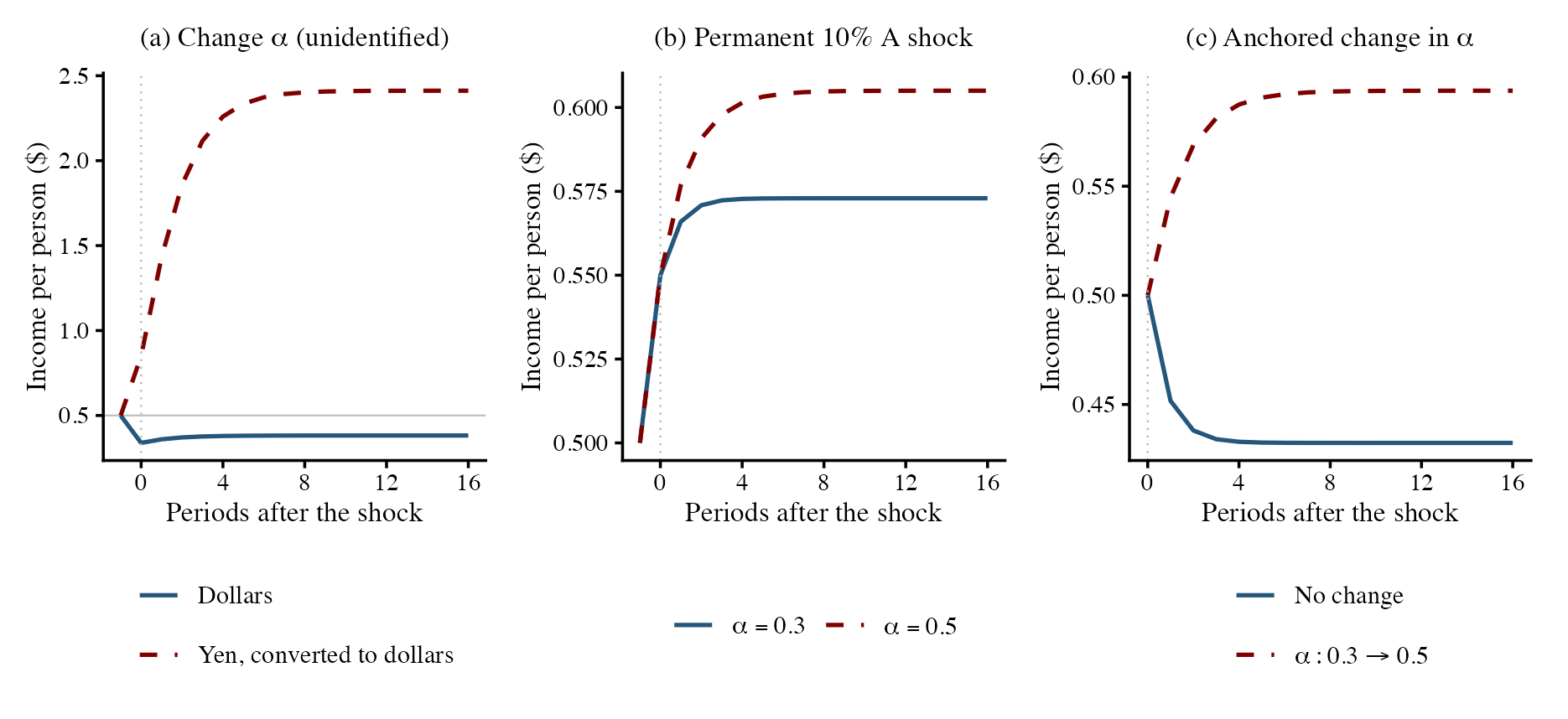
In (a), $\alpha$ rises from 0.3 to 0.5 with fitted $A$ fixed. Both calculations start from income of 50 cents, but income falls when we compute in dollars and rises when we compute in yen at 100 yen per dollar. All plotted income is in US dollars. This is the exact same scale issue emerging as in the housing example. The transition paths depend on the units.
Different baseline economies, the same shock. If we recalibrate $A$ and $k$ under the $\alpha$ change, then we remain in steady state when we change $\alpha$. Just like housing, now we must shock the economy to see how it behaves in different alpha regimes. Panel (b) then compares an unexpected permanent 10% increase in $A$ across these regimes. Each starts with income of 50 cents, but the steady-state calibration assumes that they have different baseline capital stocks because their saving rates differ. To be clear: this is a comparison of productivity shocks across economies, not a change in $\alpha$ from the same initial capital stock (I recognize this sounds unattractive). The income paths are,
\[\frac{y_t(\alpha)}{\bar y} =1.1^{\frac{1-\alpha^{t+1}}{1-\alpha}}, \qquad t\geq0.\]Both economies gain 10% on impact; capital accumulation raises the eventual gains to 14.59% and 21%. These comparisons give the same answer in either currency, just like a demand shock in the housing example. This is a silly counterfactual, however, because we don’t want to look at the world and suppose it reflects a steady state under two different technologies (this isn’t silly in the housing example, which was a static model).
The same initial capital, a change in technology. If capital $k_0$ were observed, recalibration would not need to assume that we are at a steady state, and therefore changing $\alpha$ can induce a change in the transition dynamics absent an $A$ shock (instead, think of it as a shock to the capital accumulation path).
Keeping the initial capital stock fixed and changing $\alpha$, we only need to adjust $A$ to preserve production at the baseline point (a more attractive assumption).
In panel (c), I suppose we observe $y_0$ and $k_0$, so we don’t need to assume steady state:
\[A_j=\frac{y_0}{k_0^{\alpha_j}},\qquad j\in\{0,1\}.\]Panel (c) starts both paths at income of 50 cents and capital of 20 cents. Without a change in $\alpha$, the economy is in transition, converging to its steady state: with $\alpha_0=0.3$, initial saving is 14.25 cents, below the capital stock. Now unexpectedly and permanently raise $\alpha$ to 0.5, adjusting $A$ as above. Output on impact is still 50 cents, but saving jumps to 23.75 cents. Capital now grows instead of shrinking.
Writing $x_t^{(j)}=k_t^{(j)}/k_0$, both paths obey,
\[x_0^{(j)}=1,\qquad x_{t+1}^{(j)}=0.95\alpha_j\frac{y_0}{k_0}(x_t^{(j)})^{\alpha_j}, \qquad y_t^{(j)}=y_0(x_t^{(j)})^{\alpha_j}.\]The counterfactual is the comparison of these two paths. Neither has to start in steady state, and expressing the data in yen leaves $y_0/k_0$ unchanged. So the comparison is scale free. Anchoring preserves production at the observed point, but changes investment, consumption, and subsequent output. Here we can change $\alpha$ without a separate productivity shock: the transition dynamics and the observation of $k_0$ allow us to calibrate off steady state, so the only assumption we need is that on impact, the new technology preserves current production. This gives the structure needed for a change-elasticity counterfactual to make sense in this environment.
There are other solutions. For example, task models, such as Imas and Moll (2026), specify how the aggregate production function changes as tasks are automated, providing a microfoundation for $\alpha$ which can anchor the calibration and provide the structure to make sense of a change-elasticity counterfactual (though one should be careful to check that these new features are also not scale-dependent).