Some notes on nonhomothetic CES demand
The work by Comin et al. (2021) shows how nonhomothetic CES (NH-CES) preferences are useful in capturing the smooth transition from agricultural to services observed in the data, which demand systems like Stone-Geary cannot replicate. This note derives some useful representations of the demand system for applied work and develops a toy GE model to illustrate the use in practice, by examining how the price responses from agricultural productivity increases can potentially better capture how labor reallocates across sectors following a productivity increase.
Deriving NH-CES demand
Nonhomothetic CES implicitly specifies utility for consuming a bundle $C$ through the equation,
\[\sum_i \left( {C_i \over C^{\epsilon_i}} \right)^{\sigma -1 \over \sigma} = 1\]where $C$ is maximized against the budget constraint $\sum_i P_i C_i = M$ where $M$ is income.
The resulting demand system can be written as,
\[C_i = \left( {P_i \over P} \right)^{-\sigma} \left( {M \over P} \right)^{\epsilon_i(1-\sigma) + \sigma}\]in which the price index is defined implicitly as,
\[P = \left( \sum_i \left(\left({M \over P}\right)^{\epsilon_i - 1} P_i\right)^{1-\sigma} \right)^\frac1{1- \sigma}\]This derivation is not present in the Comin et al. (2021) paper, and a more common representation of the demand system is,
\[C_i = \left( {P_i \over M} \right)^{-\sigma} C^{\epsilon_i(1-\sigma)}\]where $C$ is defined implicitly as,
\[M = \left( \sum_i \left(C^{\epsilon_i} P_i \right)^{1-\sigma} \right)^{1 \over 1 - \sigma}\]as is derived by Mestieri’s notes on the demand system.
To put the demand system in the usual CES form, which makes transparent what the price index is, and how $\epsilon_i$ affects the income elasticity, postulate the existence of a price index $P$ such that $PC=M$.
Then, the implicit equation for $C$ can be written as,
\[M = \left( \sum_i \left(\left({M \over P} \right)^{\epsilon_i} P_i \right)^{1-\sigma} \right)^{1 \over 1 - \sigma}\]Replacing $C=M/P$, and multiplying both sides by $(M/P)^{-1}$, the above equation becomes,
\[P = \left( \sum_i \left(\left({M \over P} \right)^{\epsilon_i-1} P_i \right)^{1-\sigma} \right)^{1 \over 1 - \sigma}.\]Thus, the price index is implicitly defined by the nonlinear fixed point equation above, and the price index faced by an agent depends on their income! Real income is simply $M/P$.
Using this price index, the demand function can be written as,
\[C_i = \left( {P_i \over M} \right)^{-\sigma} \left( {M \over P} \right)^{\epsilon_i(1-\sigma)}\]where multiplying by $(P/P)^{-\sigma}$ reveals,
\[C_i = \left( {P_i \over P} \right)^{-\sigma} \left( {M \over P} \right)^{\epsilon_i(1-\sigma)+\sigma}\]which is the usual CES form, with an added income elasticity.
The income elasticity of demand, $\eta_i = d \log C_i / d \log M$ is given by,
\[\eta_i = \sigma+ \epsilon_i(1-\sigma)\left[1 - {d \log P \over d \log M}\right]\]where,
\[{d \log P \over d \log M} = 1 + {d \log C \over d \log M} = 1 + \frac1{\sum_i s_i \epsilon_i},\quad s_i = {P_i C_i \over M},\]where $d \log C / d \log M$ is derived in Mestieri’s notes.
As a sanity check, it is easy to then verify that the expenditure-weighted average income elasticity is always 1,
\[\begin{align*} \sum_i s_i \eta_i &= \sum_i s_i \left( \sigma+ \epsilon_i(1-\sigma)\frac1{\sum_i s_i \epsilon_i}\right) \\ &= {\sigma } + (1-\sigma)\sum_i \left( s_i \epsilon_i \over {\sum_i s_i \epsilon_i}\right)=1. \\ \end{align*}\]This is great: this demand system has a nice, “usual” CES representation and has the normal properties of a demand system.
An example: structural change
Now let’s use the demand system in a stylized, general equilibrium setting to see its implications.
In particular, suppose there are two industries with technology, $Y_i = Z_i L_i$, and a unit mass of households deciding to which industry to allocate labor. Let $P_1$ be numeraire, so that the wage $W$ and $P_2$ are equilibrium prices pinned down by equilibrium in the labor market and goods market clearing and the allocation of labor $L_1$ and $L_2$ is endogenous and depends on $L_1 +L_2 = 1$. Note all income is wage income so $M=W$.
Wages are marginal revenue products, so $W_1 = Z_1$, and so equilibrium in the labor market requires the wage be equalized across sectors,
\[W_1 = W_2 \implies Z_1 = P_2 Z_2 \implies P_2 = Z_1/Z_2.\]Now, the only endogenous variable left is $L_1$, which is pinned down by goods market clearing, which we only need to look at for one good by Walras’ law,
\[Y_1 = \sum_i C_i(W_i)L_i.\]Since wages (income) is equalized across sectors and the mass of households is 1, this can be written as,
\[Z_1 L_1 = \left( {1 \over P} \right)^{-\sigma} \left( {W \over P} \right)^{\epsilon_1(1-\sigma)+\sigma}\]where,
\[P = \left( \left(\left({W \over P} \right)^{\epsilon_1-1} \right)^{1-\sigma} + \left(\left({W \over P} \right)^{\epsilon_2-1} {Z_1 \over Z_2} \right)^{1-\sigma} \right)^{1 \over 1 - \sigma},\]and $W=Z_1$.
Suppose now that sector 1 represents “agriculture” and sector 2 represents “industry.” I’m interested in how labor transitions from agriculture to industry as agricultural productivity increases.
As an experiment, suppose I make the following numerical assumptions, $Z_2=1$, $\epsilon_1$=0.5 and $\epsilon_2$=1.5, and $\sigma = 0.5$ (complements). Then when $Z_1=1$, the income elasticities are around 0.7 and 1.05 for the two goods.
The idea here is to generate a world where the agricultural good has an income elasticity less than 1, which is generally what you need in the structural transformation literature (see, e.g., Caselli and Coleman, 2001).
What happens to the labor force as agricultural productivity increases?
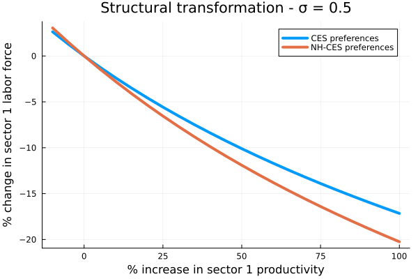
This plot shows a much more rapid reallocation of labor from agriculture to industry when the agricultural good is a necessity (and the industrial good is a luxury).
When the goods are substitutes ($\sigma = 2$),
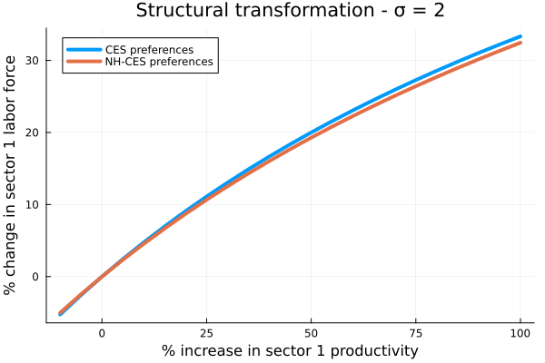
then the productivity increase in agriculture draws in labor more slowly to that sector.
Hopefully these algebraic tricks and example are useful for those seeking to use NH-CES preferences in work on structural transformation.