Growth in Cities, revisited

I recently re-read Glaeser et al.’s “Growth in CIties” (1992). They use the County Business Patterns (CBP) data to look at drivers of employment growth in US cities between 1956 and 1987.

The idea is to test different theories of agglomeration and growth. The first is the Marshall-Arrow-Romer (MAR) externality of knowledge spillovers between firms. The diffusion of production knowledge across firms within an industry amplifies the gains from innovation and generates growth. This is an intra-industry spillover and a form of external economies of scale. It also means that monopoly is good for growth. Monopolists internalize the externality and have a greater incentive to invest in innovation; competition erodes away the incentive to innovate.

The alternative view of agglomeration is Jane Jacobs’. Her book, The Economy of Cities suggests inter-industry knowledge spillovers generate growth. In short, a diverse ecosystem of different types of production finds new use for others’ ideas. Contrasting the MAR perspective on monopoly is the Schumpeterian/Porter view: competition to innovate (or otherwise perish) drives growth.

In the original paper, Ed Glaeser and coauthors find evidence that industry diversity and local competition are associated with employment growth from 1956-1987. A lot has happened since then (including updating and harmonizing the CBP), so it’s worth revisiting the question and evidence.

To that end, I quasi-replicate their exercise, looking at 1990-2015. Instead of merging counties into CBSAs, I leave counties as they are. Otherwise, I would have to worry about how to split up counties across CBSAs. Finally, it’s not clear to me whether CBSA, or commuting zone, or something else is the right aggregation. Some counties are very big and have whole cities in the (Cook for Chicago, Los Angeles for–you guessed it).

I aggregate the number of firms and employment to the NAICS-3 digit coding (after mapping SICs to 2007 NAICS). Within each 3-digit industry-by-county, I add up the number of firms and use the firm size distribution dimension of the CBP to construct employment HHI indices. The employment HHI is a proxy for how competitive a county-industry is. Then, within each county, I compute total employment and an index of industry diversity (1-industry employment share HHI). In addition, I compute average industry employment HHI and the number of firms per worker. I use these variables to summarize the competitive environment in each county. This isn’t exactly the right thing to do, since product market competition is the correct measure. Moreover, the number of firms and and HHI aren’t necessarily indicative of the competitive environment anyway, since they’re equilibrium outcomes, too. Nonetheless, we work with what we have – I’m not sending this to the Journal of Political Economy anyway.

First, just checking the raw data, I examine employment growth 1990-2015 against baseline 1990 measures of industry diversity and competition.

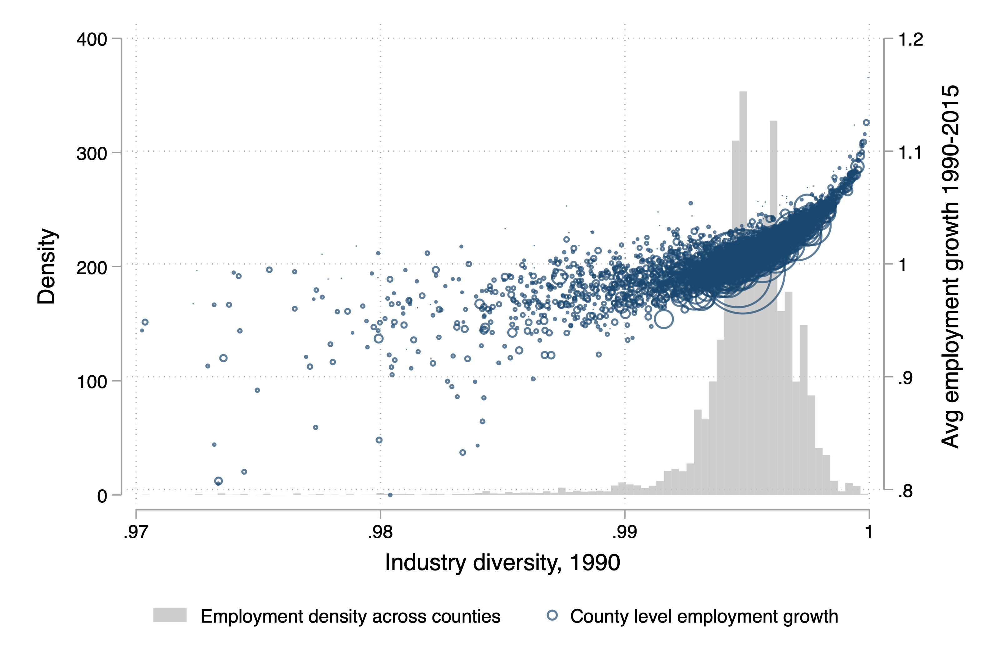
Industry diversity and employment growth are highly correlated. While there is little variation in the index, those with more diverse composition of NAICS 3-digit industries saw faster employment growth, and those with less shrank!

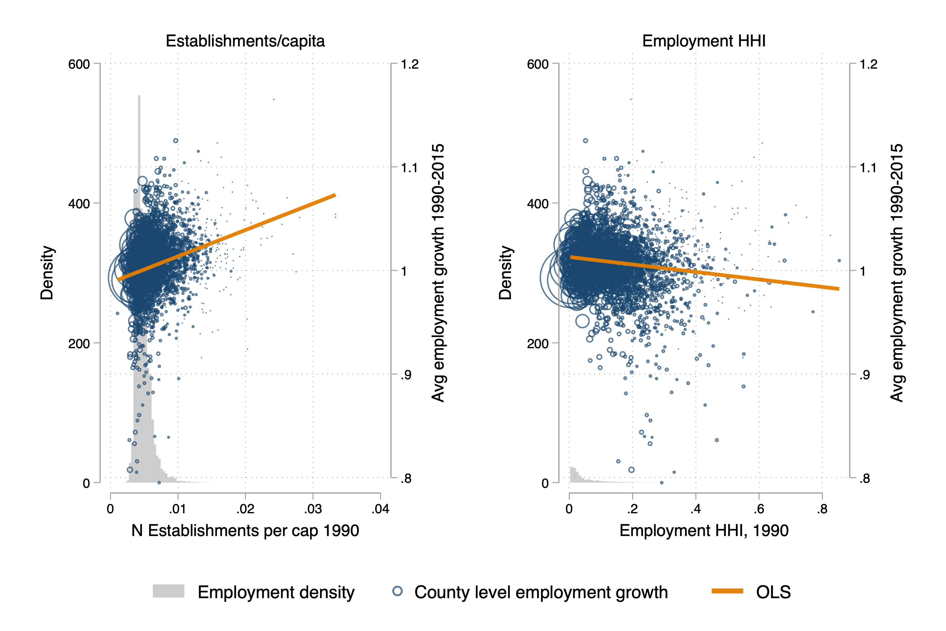
The competition story is more tenuous. While the correlations match the sign of the original paper, the relationship is weak. Counties with more competitive labor markets (more firms, lower employment HHIs) grew faster.

Now, of course, none of this is causal! However, we can do a little better than raw data correlations. These measures are correlated, and might be correlated with policy variables too. What you might want to see is scatter plots of the conditional relationship between variables, controlling for state fixed effects and the other variables. Thanks to the Frisch-Waugh-Lovell theorem, I can do this easily. In the following set of scatter plots, I residualize the X-and Y-axis variables against all the other variables discussed above, and include state fixed effects. That’s what’s below:

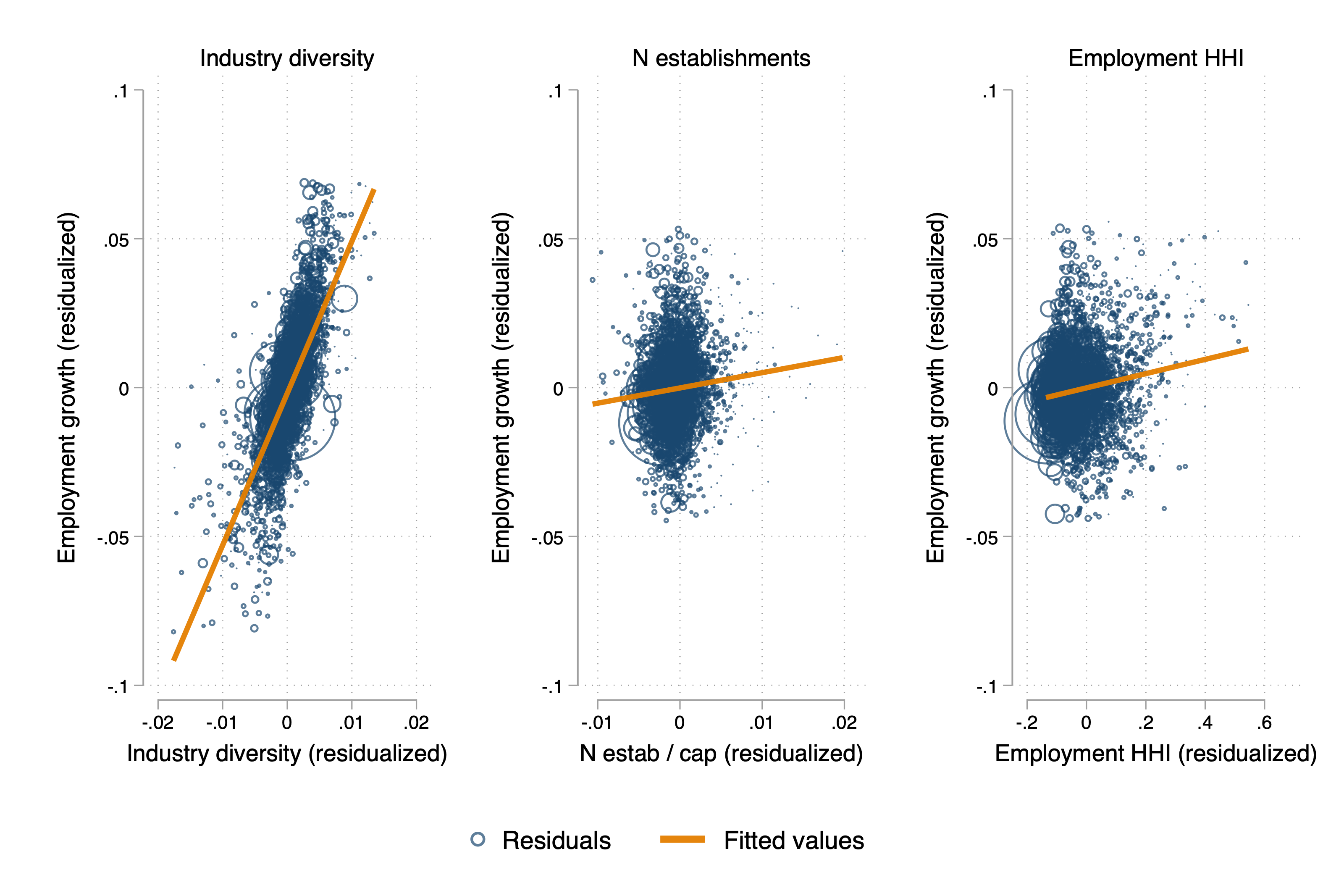
The same story holds up: industry diversity is associated with county-level employment growth (even within state!) but the competition variables don’t explain much of the residual variation. In fact, the employment HHI effect seems to reverse (though it’s likely statistically indistinguishable from zero). Of course, the local ecology of industry is a lot easier to measure than competition, so the null effects on competition could all be measurement error, anyway.

In short, “Growth in Cities” seems to hold up, at least the Jacobs vs. MAR angle. This evidence is consistent with inter-, not intra-industry spillovers driving growth. Moreover, this is consistent with Audretsch and Feldman (1999), who observe more new product introduction in less specialized areas. Of course, agglomeration is not just a dynamic externality. The existence of industrial clusters is evidence of intra-industry increasing returns – something which neither I nor the original paper deny. These scale economies may not drive industrial growth rates, however.