When is the spatial distribution of labor efficient?

In a world with agglomeration economies, it seems at first glance that the spatial distribution of labor is generically inefficient. Agglomeration is an externality, so the market doesn’t provide enough of it. We also might worry about congestion forces, negative urban externalities which the market overprovides. I think since the 70s, the consensus has shifted from thinking there’s too much congestion to thinking there isn’t enough agglomeration.

Kline and Moretti (2014) and Glaeser and Gottlieb (2008) both write down spatial models where surprisingly, the competitive equilibrium is efficient. However, Fajgelbaum and Gaubert (2020) show that this is due to both an inability for the planner to make transfers across regions and a constant-elasticity agglomeration function. Accounting for this, in their model, the spatial distribution is inefficient, but they restrict their planner with a spatial mobility constraint. Rossi-Hansberg et al. (2022) write down a model with heterogeneous workers that generates different agglomeration elasticities in different places. As the social and private value of labor differs across space, their planner’s allocation can be implemented with wage subsidies that reallocate labor across space.

All this stuff works with specific models and are a bit unclear about welfare and the constraint the hypothetical planner faces, so let me propose a simple but general model to highlight the role of agglomeration and transfers to illustrate when the competitive equilibrium is efficient. I’ll exposit now this model now.

Environment

Suppose there are two regions (or industries), 1 and 2, to which a unit mass of labor inelastically supplies labor. A share of households $x$, allocated to region 1, receive utility $u_1(x,c_1)$, while the $1-x$ remainder are allocated to region 2 and receive utility $u_2(1-x,c_2)$ when consumption levels are $c_1$ and $c_2$.

Efficiency when there are no transfers across regions

Without transfers across regions, consumption equals output in each region, $c_1 = y_1(x)$ and $c_2=y_2(x)$, meaning utility can be written indirectly as,

and the same for $u_2$.

In a competitive environment, spatial equilibrium most hold, which requires utility equalization across space:

The planner wants to maximize welfare, so their problem is,

where the resource constraint is embedded in their objective. The planner’s first order conditions are,

Note that the second term can be written using elasticities, $\varepsilon_1 \tilde u_1 - \varepsilon_2 \tilde u_2$. When $\varepsilon_1 = \varepsilon_2 = \varepsilon$ and is a real number (i.e., utility is constant-elasticity in the size of the region), then the planner’s FOC can be written as,

which implies the decentralized solution,

i.e., the spatial equilibrium holds. When utility is constant elasticity but varies across regions,

When congestion overall dominates, but region 1 has stronger agglomeration forces, $0>\varepsilon_1>\varepsilon_2$ and therefore the planner prefers to have $x$ set above the market level.

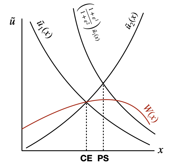
This is visible in the above figure: spatial equilibrium, the competitive equilibrium (CE) underprovides labor to the region with greater welfare relative to the planner’s solution (PS). $W(x)$ represents the welfare function, which peaks to the right of the competitive solution.

Efficiency with transfers

Suppose there are transfers across regions, and that in the competitive economy, market clearing for goods happens without frictions across regions,

Despite trade, households are still on their budget constraint, $y_1(x)=c_1$. Spatial equilibrium still holds, so that,

i.e., allowing free trade does not affect the competitive allocation! However, the planner can internalize the externality that $\partial y_i(x) / \partial x > 0$ and reallocate labor to maximize output and then use transfers to equate marginal utilities of income across regions.

That is, the planner solves,

Letting $\mu$ be the Lagrange multiplier on the resource constraint, so that the FOC on $x$ is,

Or,

Now, with transfers, it is clear that the spatial equilibrium has an additional wedge which further incentivizes the planner to distort the allocation of labor across regions.