Messing around with Brancaccio et al. (2019)

NB: This is a post primarily for me to reference but thought it served as a public good

The latest Frisch medal winner, Geography, Transportation, and Endogenous Trade Costs by Giulia Brancaccio and coauthors presents a spatial search model that endogenizes trade costs. They start from the observation that the market for ships is rife with search frictions, and there’s a lot of trips carrying ballast (as opposed to cargo) on the open seas. Ships travel from port to port looking for dry bulk to transport elsewhere. Because search is costly, the negotiated price of a trip depends not only on the value of the cargo, but also on the ship’s ease of search at the destination once the cargo is offloaded.

This paper is a big deal because it endogenizes trade costs with ‘microfoundations’ that plausibly match the actual organization of the shipping industry, and moreover those costs depends on the spatial organization of ports. I like it because it provides a quantitative foundation for spatial search that could plausibly be extended to other settings, or embedded in a general equilibrium trade model.

The guts of the model, and how shipping roughly works, are as follows:

• Ships transport freight from port to port. They are (basically) homogenous and in fixed supply.
• Ships arrive in ports where they meet with exporters, and negotiate a price for freight to be shipped elsewhere.
• If a ship cannot or does not want to meet with an exporter in a port, they can travel carrying ballast (valueless cargo that helps keep the ship stable on the open seas) to another port.
• Travel? It’s costly.

The model

This is a slightly simplified version of the model presented in the paper. In the model, locations are indexed by $i$ or $j$. Time is discrete, but they only consider the steady state of the model, so I’m dropping all the time notation of the paper. The state variables in the model are the spatial distribution of ships $s_i$ and exporters $e_i$, which come from a pool of potential exporters $\mathcal E_i$ at every location.

Everyone discounts using the factor $\beta$. Trade costs are $\tau_{ij}$. When a ship is sailing from $i$ to $j$, it arrives at $j$ with probability $d_{ij}$. When a ship is sailing, its value function is,

The value of arriving in a port and searching for an exporter depends on flow search costs and the probability of meeting an exporter, $\lambda_i$, as well as the expected value of being unmatched, $U_i$,

When a ship is unmatched, it decides whether to remain in port $i$ or sail with ballast elsewhere. This is a discrete choice problem, so we employ a trick of making this decision subject to a T1EV shock $\epsilon_j$, so that,

Which gives T1EV choice probabilities, $P_{ij} \propto \exp(V_{ij}/\sigma)$.

The value of freight along route $i\rightarrow j$ is $r_{ij}$. Exporters in $i$ that send freight to $j$ and match with a ship earn $r_{ij}$ but pay $\tau_{ij}$. An exporter that decides to enter survives with probability $\delta$, and matches a ship with probability $\lambda_i^e$. The value of remaining unmatched is,

In each period, exporters among the $\mathcal E_i$ potential entrants decide whether to enter, along which route to enter if so, or to get the value of the outside option. Shipping from $i$ to $j$ is costly in excess of what’s paid to the ship, due to unmodelled frictions via $\kappa_{ij}$. Again this discrete choice is subject to T1EV shocks $\epsilon^e$, so that the probability of exporting $i$ to $j$, ${P_{ij}^e} \propto \exp(U_{ij}^e - \kappa_{ij})$.

Trade costs are determined through Nash bargaining with weight $\gamma$, so that they solve,

By solving for $U_{ij}^e$, it can be shown that, $\tau_{ij} = (1-\mu_i)(U_i - V_{ij}) + \mu_i r_{ij}$ where $\mu_i$ is an equilibrium constant that depends on the matching probabilities and the model primitives.

Trade flows still have a gravity-flavor in the model: an endogeneous origin component that is governed by local outside options, an endogenous destination component on the value of search at the destination, and exogenous bilateral shifters. However, these components combine nonlinearly, so that the log-linear bilateral term contains both endogenous origin and destination components. To see this, first rearrange $V_{ij}$,

Then plug this into the price equation

Substituting for $U_{ij}^e$ into the exporter probabiilities to derive the trade flows $X_{ij}$, it’s easy to see that,

Where do the match probabilities come from? Some matching technology $m_i(s_i,e_i)$ so that $\lambda_i = m_i/s_i$ and $\lambda_i^e = m_i/e_i$.

In equilibrium, values must satisfy the Bellman equations above, choice probabilities must be defined using the Bellman satisfying values, and $s_i$ and $e_i$, and the number of trips along routes $i,j$, $s_{ij}$ must all be at their steady state values. For ships,

For exporters,

and for ships,

Solving the model

Knowing $s_i,e_i$, it is straightforward to solve for $V_i$ through fixed point iteration. The key is to then correctly update $s_i$ and $e_i$ so as to solve the model’s equilibrium. Following the paper’s online appendix, the solution algorithm consists of an inner loop (solve Bellmans) and outer loop (update stationary distribution of ships and exporters).

Like a maniac, I solve the model for some artificial parameters in R. Yell at me to use Julia later.

Let’s set up the environment,

set.seed(82422)
# parameters
beta = 0.975; delta = 0.8; gamma = 0.5; sigma = 3

# fictious locations
N <- 13 # number of countries
S <- N*300 # number of boats
xy <- matrix(runif(2*N),N,2) # locations in the unit square
dists <- as.matrix(dist(xy))

Now, I need to set up the potential exporters $\mathcal E_i$, the costs $c_i^w$ and $c_{ij}^s$, and $\kappa_{ij}$, and the revenues $r_{ij}$ and the arrival probabilities $d_{ij}$. I’ll make these a function of distances. For revenue, I’ll write $r_{ij}=r_i u_{ij} r_j$.

# origin components
u_i <- rnorm(N) # make size and revenue correlated
potential_exporters <- round( matrix(exp(5+0.75*u_i),1,N) ) # log normal
port_costs <- matrix(1,1,N) # no spatial het here
ri <- matrix( pmax(exp(1+0.25*(0.75*u_i + 0.25*rnorm(N))),1),1,N) # bound below by 1

# bilateral
kappa_ij <- exp(2*dists) - 1 # exogenous trade costs
u_ij <- matrix( exp(rnorm(N^2)), N,N) # bilateral revenue shifter
u_ij = 0.5*u_ij + 0.5*t(u_ij) # make symmetric
r_ij <- t(ri) %*% ri * u_ij
d_ij <- 0.75*exp(-2*dists) + 0.25*matrix(runif(N^2),N,N)
sailing_costs <- matrix(1,N,N) # no spatial het here, either

We also need a matching function. Let’s go with Cobb Douglas, enforce a min, and have no spatial heterogeniety,

matches <- function(s,e){
  return(
    pmin(0.5 * s^0.5 * e^0.5,s,e)
  )
}

In the inner loop, I solve for $V_i$.

solve_Vi <- function(Vi_init,si,ei){
  
  tol = 1e-8; error = tol + 1
  iter = 0; maxIter = 20
  
  #Vi0 <- matrix(Vi_init,1,N)
  while(error > tol & iter < maxIter){
    
    # construct V_ij
    V_ij = ( - sailing_costs + d_ij * beta * matrix(t(Vi0),N,N) )/(1 - beta*(1-d_ij))
    diag(V_ij) <- 0
    
    # construct U_i
    U_i = sigma*log( exp( beta/sigma*Vi0 ) + rowSums(exp(V_ij/sigma)) ) - sigma*digamma(1) # euler's constant
    
    # compute prices
    lambda_e = matches(si,ei)/ei
    mu_i = (1-gamma)*(1-beta*delta)/(1 - beta * delta * (1 - gamma*lambda_e) )
    mu_i <- matrix(t(mu_i),N,N)
    
    tau_ij = (1-mu_i)*(matrix(U_i,N,N) - V_ij) + mu_i * r_ij
    diag(tau_ij) <- 0
    
    # compute P_ij^e
    alpha <- beta*delta*lambda_e/(1-beta*delta*(1-lambda_e)) # eq constant
    alpha <- matrix(alpha,N,N)
    P_ije <- exp(alpha*(r_ij - tau_ij) - kappa_ij)
    diag(P_ije) <- 0
    P_ije <- P_ije / (1 + rowSums(P_ije))
    P_ije_cond <- P_ije / rowSums(P_ije) # P_ij^e / (1 - P_i0^e )
    
    # update Vi0
    lambda <- matches(si,ei)/si
    Vi1 <- -port_costs + lambda*( rowSums(P_ije_cond*(tau_ij + V_ij) ) ) + (1-lambda)*U_i
    
    # update convergence criteria
    error <- max(abs(Vi0-Vi1))
    #message(error)
    Vi0 <- Vi1
    iter <- iter + 1
    
  }
  
  # get ballasting probabilities
  diag(V_ij) <- Vi1
  Pij <- exp(V_ij/sigma)
  Pij <- Pij / rowSums(Pij)
  
  # return
  return(
    list(
      Pij = Pij,
      Vi = Vi1,
      Pije = P_ije,
      tau_ij = tau_ij
    )
  )
  
}

The outer loop is simple,

tol = 1e-3; error = 1+tol
iter = 0; maxIter = 250
update = 0.5

# initialize
e0 <- 0.5 * potential_exporters/(1-delta)
s0 <- matrix(S/N,1,N)

Vi0 <- matrix(1,1,N)
while(error>tol & iter < maxIter){
  
  inner_loop <- solve_Vi(Vi0,s0,e0)
  
  P_ije <- inner_loop$Pije; Pije_cond <- P_ije / rowSums(P_ije)
  P_ij <- inner_loop$Pij
  
  e1 <- delta*(e0 - matches(s0,e0)) + potential_exporters*rowSums(P_ije)
  s1 <- t(P_ij) %*% t(s0 - matches(s0,e0)) + t(Pije_cond) %*% t(matches(s0,e0))
  s1 <- t(s1)
  Vi0 <- inner_loop$Vi
  
  error <- max( max(abs(s1-s0)), max(abs(e1-e0)) )
  iter <- iter + 1
  message(paste0("iter: "),toString(iter),", error: ",toString(error))
  
  # update
  s0 <- s0 + update*(s1-s0)
  e0 <- e0 + update*(e1-e0)
  
}

And that’s the model!

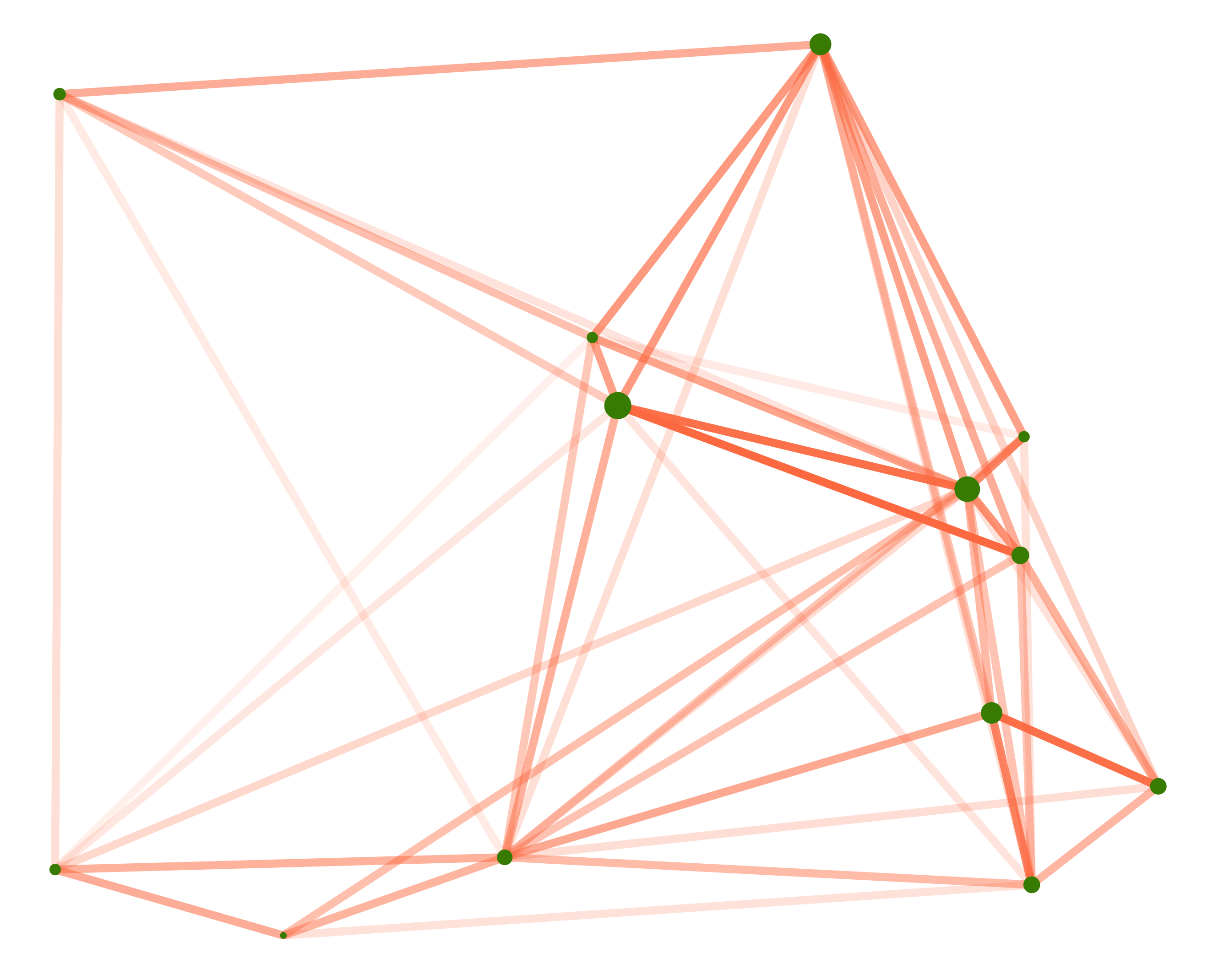
Here’s the simulated trade network made using the ggraph package. Line transparency reflects bilateral shipping volume, and the locations are the same used to solve the model above.

The paper ends with the quote, “embedding our setup within a general equilibrium framework that endogenizes product prices is an exciting avenue for future research.” I agree and look forward to reading those papers.