Some thoughts on Diffusion-State-Distance

I’ve thought for a while that Diffusion-State-Distance (DSD), a metric that applies to graphs, would be a good basis for a model-based (social) network clustering exercise. The metric was first introduced in Cao et al. (2013), a computational biology paper I encountered in undergrad (some of the coauthors are from the Tufts CS department) that has hasn’t really been picked up in the literature since, outside a handful of extensions.

The basic exercise is that two nodes in a network ought to be thought of as similar if they diffuse information throughout the network in a similar way; e.g., if the probability a given received message is equally likely to have originated at either node.

To fix ideas and notation, let $P$ be a probability transition matrix associated with some network described by the adjacency matrix $A$, $P = D^{-1} A $, $D = \operatorname{diag}(\operatorname{colSums}(A))$, so that $P_{ij} = Pr($message sent by $i$ is received by $j)$.

The original DSD paper considers the expected number of messages to arrive after $t$ steps. Switching $i$ and $j$ notation (for reasons to be made clear soon):

Then a natural measure of how distant $j$ and some other node $k$ are, from $i$’s perspective, is,

The clever trick of the DSD paper is to show that the limit of this, as $T\rightarrow\infty$ exists and can be written down. First, let $W$ be a matrix whose rows are the steady state probabilities, $W_{i\cdot} = \pi$, $P\pi = \pi$. Note then that $(e_j - e_k)’ W = \pi - \pi=0$ for any $j,k$. Adding up over the $e_i$s and breaking open the sum we have,

Now, another insight is that $PW = W \implies P^t W = W$ and also $W P = W$, so canceling $W$ terms $(P-W)^t = P^t-W$. and so we can subtract $W$ off each term in the above without affecting the norm,

and then using our new fun fact,

The standard geometric series analogous fact is that this sum converges if the spectral radius $\rho(\cdot)$ of $P-W$ is less than 1.

It is. The following is my proof, not the one in the Cao et al paper, which is a bit more difficult. First, we need $P$ to be diagonalizable, so we’re working with a connected graph. Then, recall: $\lim_{k\rightarrow\infty} P^k = W$ and $(P-W)^k = P^k - W$. So $\lim_{k\rightarrow\infty} (P-W)^k = 0$. Diagonalizing $(P-W)^k = U V^k U^{-1}$, we need the eigenvalues $\lambda_n$ along the diagonal of $V$ to all go to zero for the limit to hold, meaning $ \mid\lambda_n\mid<1$and therefore $\rho(P-W) = \max_n \mid \lambda_n \mid<1$. QED.

Averaging across $e_i$s, and using the fact that the sum converges, the distance between $j$ and $k$ then is,

where DSD is the measure proposed in the paper. It is a metric: obeying the triangle inequality, symmetry, and $DSD(j,k)=0\implies j=k$. Note the choice of norm didn’t actually matter; one could use the $2$-norm, for example.

An Example

The following uses the igraph package,

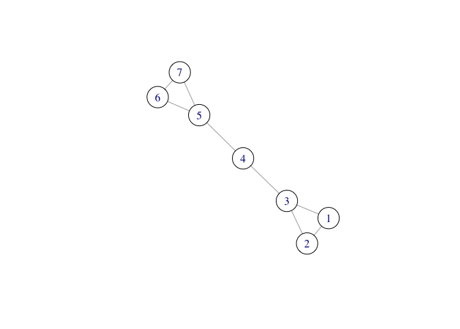
# will create a simple 7-node graph with two "clusters"
c12 <- c(1,1,1,0,0,0,0)
c3 <- c(1,1,1,1,0,0,0)
c4 <- c(0,0,1,1,1,0,0)
A <- matrix(c(c12,c12,c3,c4,rev(c3),rev(c12),rev(c12)),7,7)
gr <- igraph::graph.adjacency(A, mode="undirected")
plot(simplify(gr),vertex.size=25,vertex.color='white')

Then let’s define a function to compute DSD

# first, a function that gives basis vectors
basis <- function(i,n){
  v <- as.vector(matrix(0,n,1))
  v[i] <- 1
  return(v)
}

DSD <- function(A){
  # create probability transition matrix
  P <- diag(1/colSums(A)) %*% A
  n <- dim(P)[1]
  
  # solve for steady state via linear system
  M <- rbind(t(diag(n)-P),1)
  pi <- solve(t(M)%*%M,t(M)%*%c(0 * 1:n, 1))
  
  # create W matrix, solve (I-P+W)^{-1}
  W <- matrix(1,n,1) %*% t(pi)
  dsd.matrix <- solve( diag(n) - P + W )
  
  # compute the distances between all pairs
  out <- matrix(0,n,n)
  for (ii in 1:n) {
    for (jj in 1:ii) {
    if(ii!=jj){
      dist <- norm( ( basis(ii,n)-basis(jj,n) ) %*% dsd.matrix , type="1")
      out[ii,jj] <- out[jj,ii] <- dist
      }
    if(ii==jj){
      out[ii,jj] <- out[jj,ii] <- 0
    }
    }
  }
  return(out)
}

Now consider the heatmap,

heatmap(DSD(A),Rowv=NA,Colv=NA)

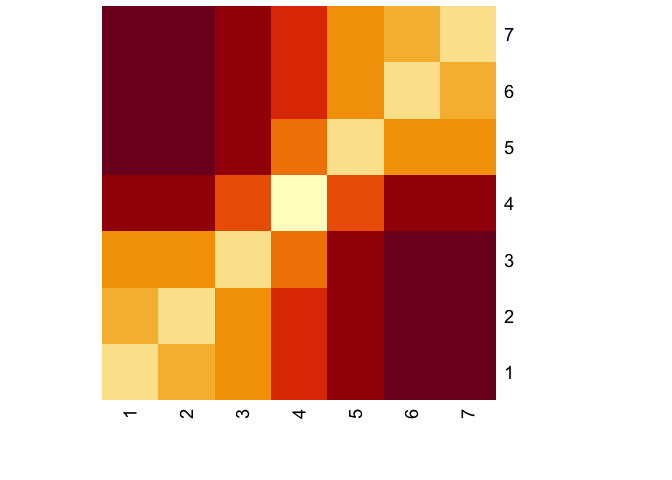
Visual inspection is pretty informative on whether DSD finds the clusters.

Constructing an embedding

Now, once you have a distance matrix, it’s not immediately clear how one ought recover a clustering. Most clustering algorithms rely on some mapping into Euclidean space to use something like a $k$-means algorithm. With just a distance matrix, you could try to implement something like k-medoids or some sort of distance-based hierarchical clustering algorithm.

These are all black boxes I don’t particularly like, so an alternate approach is to try and reconstruct points in Euclidean space whose pairwise distances match those in the DSD matrix.

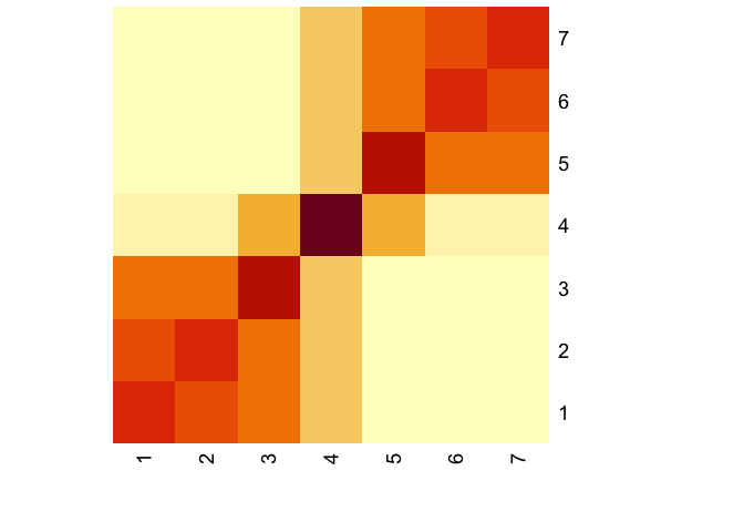
Recall the DSD formula,

so reconstructing any embedding amounts to performing some dimensionality reduction on $(I-P+W)^{-1}$. It’s worth staring at that matrix, for a second too, because the clusters are evident:

P <- diag(1/colSums(A)) %*% A
n <- dim(P)[1]
# solve for steady state of P
M <- rbind(t(diag(n)-P),1)
pi <- solve(t(M)%*%M,t(M)%*%c(0 * 1:n, 1))
# create W matrix, solve (I-P+W)^{-1}
W <- matrix(1,7,1) %*% t(pi)
dsd.matrix <- solve( diag(n) - P + W )
heatmap(dsd.matrix , Rowv=NA,Colv=NA)

The simplest Euclidean embedding would be to find the 1-dimensional embedding, and then cluster from there. This clever stackexchange post spells out exactly how to do this, which I’ll recap here:

We want to write,

where $\beta_i$ will be the 1d coordinate of node $i$. Let $X$ be a matrix whose $m$th row is $e_i - e_j$. Then we can specify the regression equation,

to recover the $\beta$s. An open question is what, exactly, we think the error term represents here. Perhaps it’s that DSD is measured with noise, but I think one has to be really careful thinking about from where that noise stems – because if it’s unsampled connections that could change the whole topology of the network, so there has to be some underlying structure that you believe is being held fixed when you observe a network.

Finally, there’s the question of what the dimension $\beta$ represents.

Aspirationally, a nice model might be along the lines of there being some underlying typespace for nodes indexed by $\beta \in \mathbb{R}$ and $Pr(i$ forms a link with $j)\propto \exp(-| \beta_i - \beta_j |)$, and then if potentially if set up right this procedure is recovering the index.

Creating the data for this:

D <- DSD(A)
n <- dim(D)[1]

# OLS
m <- 0.5*n*(n-1)+n
Dij = matrix(0,m,1)
X <- matrix(0,m,n)
z <- 0 # counter
for(jj in 1:n){
  for(ii in jj:n){
    z <- z + 1
    Dij[z,] <- D[ii,jj]
    X[z,] <- basis(jj,n) - basis(ii,n)
  }
}

And then estimating, both using OLS and then with a little regularization:

lm(Dij ~ 0 + X)

## 
## Call:
## lm(formula = Dij ~ 0 + X)
## 
## Coefficients:
##     X1      X2      X3      X4      X5      X6      X7  
## 5.8634  5.5776  4.6832  2.9317  1.1801  0.2857      NA

fit <- glmnet(X,Dij,alpha=0.5,intercept=FALSE)
coef(fit, s = 0.01)

## 8 x 1 sparse Matrix of class "dgCMatrix"
##                     1
## (Intercept)  .       
## V1           2.915209
## V2           2.628397
## V3           1.734839
## V4           .       
## V5          -1.734343
## V6          -2.627864
## V7          -2.914646

So this does a pretty good job at finding the clusters in this little example.

Recovering a Stochastic Block Model

The example so far has been pretty stylized. Let’s simulate a SBM with 2 clusters and many nodes.

pm <- cbind( c(.1, .001), c(.001, .05) )
sbm <- sample_sbm(200, pref.matrix=pm, block.sizes=c(60,140))
image(as_adjacency_matrix(sbm))

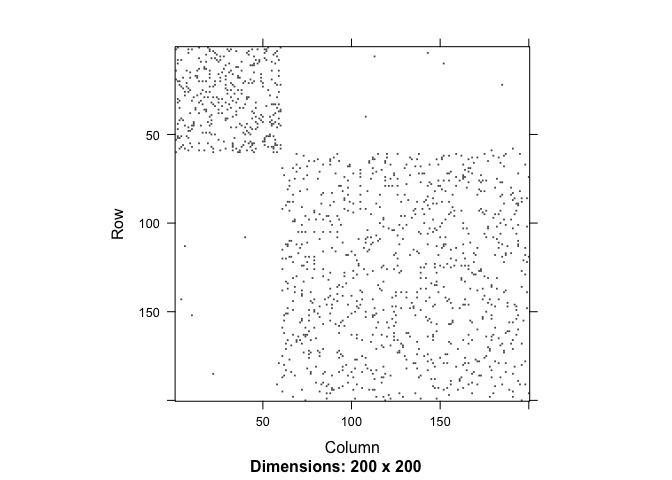
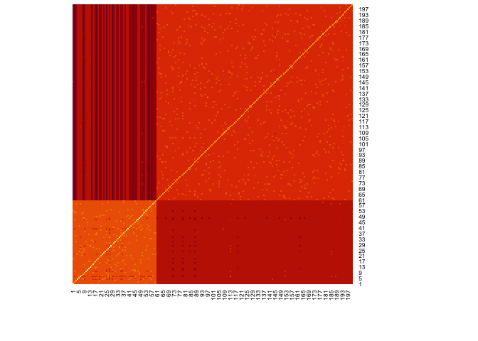
What does the DSD matrix look like?

Asbm <- as_adjacency_matrix(sbm,sparse=FALSE)
# get connected component, from the ggm package
cc <- conComp(Asbm) 
Asbm <- Asbm[cc==1,cc==1]
Dsbm <- DSD(Asbm)
heatmap(Dsbm,Rowv=NA,Colv=NA)

and then trying to line up the points via OLS,

n <- dim(Dsbm)[1]

# OLS
m <- 0.5*n*(n-1)+n # size of diagonal
Dij = matrix(0,m,1)
X <- matrix(0,m,n)
z <- 0 # counter
for(jj in 1:n){
  for(ii in jj:n){
    z <- z + 1
    Dij[z,] <-  Dsbm[ii,jj] 
    X[z,] <- basis(jj,n) - basis(ii,n)
  }
}
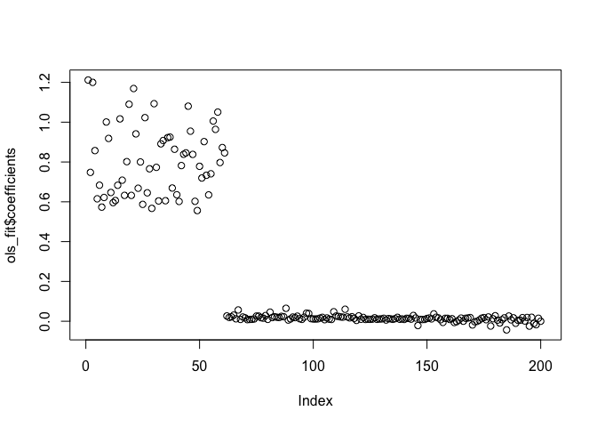
ols_fit <- lm(Dij ~ X)
plot(ols_fit$coefficients)