Power Laws and Benford's Law

In the class of things that display universality, power laws occupy a special place in the academic imagination. Those who encounter them return babbling like a character in a Lovecraft story. Perhaps this shouldn’t be a surprise: their simplicity belies the fact that they are often difficult to explain theoretically, and their ubiuquity carries the type eldritch horror that’s par for the course when uncovering an inexplicable secret to the universe. Some examples:

• In economics, Xavier Gabaix, who has an early paper on the eerie empirical regularity that the size distribution of cities follows Zipf’s law has a detailed paper on power laws in finance.
• Sandpiles (like, literally dropping grains of sand onto a plain and seeing if stable pyramids form) have cluster sizes distributed by a power law.
• The number of connections each node has in a social network is Pareto distributed – this is proven in the classic Barabasi-Albert model.
• The metabolic rate of an animal is $\propto$ animal’s mass$^{3/4}$ (Kleiber’s law).
• Et cetera; Geoffrey West has a whole book on this; there’s even a Wikipedia list.

What’s going is is that power laws are universal in a dynamical systems sense – that the order these “laws” describe is reflective of something that’s inherent to life or complex systems in general. As Terry Tao notes in his post on universality, a key feature of these kinds of laws is compatibility, that one describes the other.

Benford’s Law

One “law” related to power laws is Benford’s law, which describes the uncomfortable regularity at which leading digits of numbers – really, any numbers – follow a known distribution: In nature, 1s appear about 30% of the time, 2s 17.5%, etc, declining exponentially.

In the episode “Digits” of the Netflix science show “Connected,” Jennifer Golbeck (Prof at U Maryland’s i-School) talks about her paper that Benford’s law applies to friend and follower count on social networks. Since the degree distribution in social networks is likely governed by a power law (this is controversial, here’s a Quanta article and Barabasi’s reply), I wondered if just drawing the first digits of numbers from a power law would automatically give rise to Benfordness.

Experimenting in R, I use the Pareto distribution, $x_i \sim {\alpha x_m^\alpha \over x^{\alpha+1}},$ where I fix $x_m=1$ (this shouldn’t matter, as the properties are power laws are “scale-free”), and experiment with $\alpha$. Note here our power law is that $x_i \sim \alpha x^{-(\alpha+1)}$.

I then follow this procedure:

• For a given $\alpha$, draw $N=150,000$ iid draws from the Pareto distribution, i.e.,

# inverse of pareto cdf
Finv <- function(y,xm,alpha){
  return((1/xm)*(1-y)^(-1/alpha))
}
# draw N uniform samples
u <- runif(N)
# create pareto draws
pareto_draws <- sapply(u,Finv,xm=1,alpha=my_alpha)

• Record the first digit of each draw
• Compute the fraction of the sample with leading digit $1,…,9$.
• Compute the Euclidean distance of that vector against Benford’s law, that the digits are distributed $P(x=d)=\log_{10}{d+1 \over d}$. In the figure below, I call this $|\text{x-y}|$.

What we get is the following:

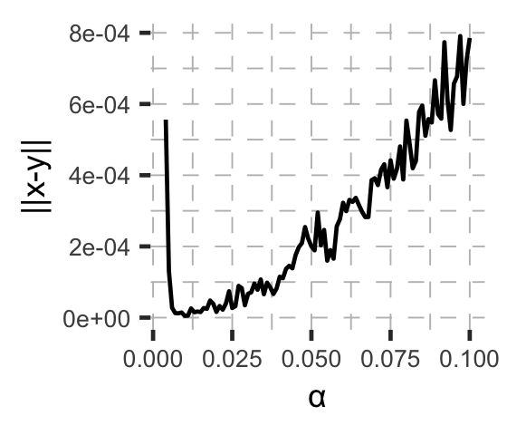
We get the Benford distribution almost exactly when using $\alpha=0.01$,

This is, IMO, extremely surprising. The city size distribution, for example, is known to follow Benford’s law, see, e.g., this site. Yet the city size $\alpha$ is generally estimated at around $\alpha=1$, (see this Gabaix and Ioannides paper, for reference).

In this numerical experiment, at $\alpha=1$, we observe superbenfordness. That is,

Downloading the 2010 U.S. cities and towns census estimates, we see the distribution of leading digits in city size is roughly Benford,

We have found an inconsistency: Pareto distributions only produce Benford’s Law for $\alpha \rightarrow 0$, and Zipf’s Law for cities says the Pareto exponent for U.S. cities is roughly $\alpha=1$, and yet the U.S. city size distribution appears to obey Benford’s law.

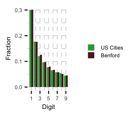
This is consistent with the observation that Zipf’s law for U.S. cities does not hold, and that if anything, the U.S. city size distribution is only Pareto in one tail.